Can we provide a DSP core that is designed to meet all of our customers' unique design requirements. Sometimes the kernel will be too big, too small or not fast enough. Sometimes we develop a core that exactly meets our customers' needs and quickly launches under the CORE GeneratorTM trademark. But even in this case, customers still want a specific set of DSP functions, and there is no time to delay. In these cases, I often advise them to customize their DSP capabilities using the interpolation lookup table in our device.
A lookup table (LUT) is essentially a storage element that can "find" the output based on any given combination of input states to ensure that each input has an exact output. Using LUTs to implement DSP functions has some significant advantages:
You can change the LUT content with a high level abstraction programming language such as MATLAB® or Simulink®.
You can design a DSP function to run mathematical functions that are extremely difficult with discrete logic operations, such as ly="log"(x), y=exp(x), y=1/x, y=sin(x) Wait.
The LUT can also easily perform complex mathematical functions that may require excessive FPGA resources in terms of configurable logic block (CLB) chips, as well as embedded multiply cells or DSP48 programmable multiply-accumulate (MAC) cells.
However, using LUTs in this way will of course have some drawbacks. When you use the LUT to implement DSP functions, you must use block RAM (BRAM) components. If the function y="sqrt"(x) is executed (where x is a 16-bit input and y is an 18-bit output), each variable requires approximately 64 18KB BRAM cells. If, for example, your goal is to implement a miniaturized Spartan® device, or if you have too many operations to perform and you cannot save 64 BRAM cells for each variable, we recommend that you abandon this method that requires such a large number of BRAM cells. From the perspective of system architecture, this method is too costly.
The interpolated LUT method not only has the advantages of the LUT method in implementing DSP functions, but also does not require the use of too many BRAM cells. In this way, you can linearly interpolate from a continuous output from a smaller LUT (for example, a 1000-word LUT) to simulate a larger capacity LUT. This way, you can achieve a higher numerical resolution than the 1000 word LUT. In addition, with this method, only one BRAM, one embedded multiplier (or DSP48), and a few CLB chips can implement the control logic, so the cost of using the LUT becomes more rational. Moreover, from the point of view of the signal-to-noise ratio, the numerical accuracy is also very satisfactory.
Of course, applying the interpolation LUT (ILUT) method requires some skill. For example, when this method is used to execute the y=sqrt(x) function, the performance of the ILUT in terms of area occupancy, timing, and numerical precision can be clearly displayed. Let's take a look at this example first, and then I will explain some examples of how to use this method to meet the different needs of customers, such as linearizing the sensor with non-linear transfer functions and implementing adaptive finite impulse response ( FIR) Filter to eliminate speckle noise on Synthetic Aperture Radar (SAR) images.
Design with System Generator for DSP
To implement the DPS algorithm on Xilinx FPGAs, I used the System Generator for DSP design and synthesis tool using MathWorks Simulink's model-based design methodology. System Generator benefits from Xilinx's DSP blockset in the Simulink environment, which automatically calls the CORE Generator to generate highly optimized netlists for DSP building blocks. Simulink is a double-precision floating-point design tool, while System Generator is a fixed-point computing tool. In any case, you can use the two tools together to define the total number of bits per signal and the binary position of each signal, so that the scores are handled in a fixed-point operation. The simulation results are accurate and bit-true, so you can easily compare them to MATLAB scripts or floating-point reference values ​​generated by Simulink blocks to check for quantization errors.
Figure 1 shows the top-level structure of the ILUT scheme in System Generator. To make this method as general as possible, assume that the input variable x in nx=16 bits has a value range of 0≤x<1, so its format is “unsigned 16 bits plus 16 bits to the right of the binary pointâ€. It is called Ufix_16_16 format. The Most Significant Bit (MSB) and Least Significant Bit (LSB) modules correspond to the highest bit of the input data nb=10 and the lowest bit of nx-nb=6, respectively. These signals are named x0 and dx. The y=sqrt(x) output is represented by a ny=17-bit binary number in the format: Ufix_17_17.
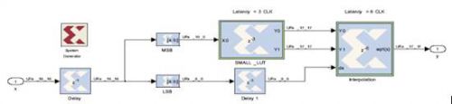
Figure 1. Top-level block diagram of the interpolation lookup table in System Generator for DSP
Figure 2 shows the deployment steps for a 1000-word small-capacity LUT through a dual-port RAM module. Since the module is read-only memory, the Boolean constant module We_const forces the write to zero. Signals X0 and X0+1 are used as the next two addresses on the ROM table. The zero constant of the Data_const module defines the size of any ROM word (ie ny in this example).
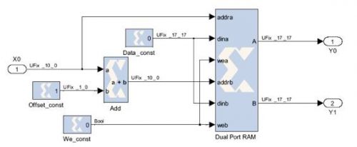
Figure 2 Small capacity LUT diagram in System Generator for DSP
The following formula shows how to insert a point with coordinates (x, y) between two known points (x0, y0) and (x1, y1) with x0 being the most significant bit of x:
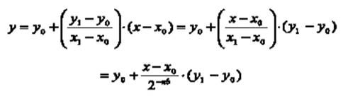
Note that X1 and X0 are the adjacent addresses of this small-capacity LUT with only one least significant bit separated. Since the address space of this small-capacity LUT is the nb bit, the value of the LSB is 2-nb.
The interpolation step is shown in Figure 3. The "Reinterpret" module can change the dx=x-x0 signal without changing the binary representation. It resets the binary point (from UFix_6_0 to UFix_6_6 format) and outputs a fraction of the nx-nb bit binary number to calculate the value of (x-x0)/2-nb.
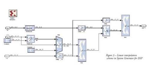
Figure 3 Linear inside illustration of System Generator for DSP
From a hardware perspective, these modules are not occupied. In general (and depending on the type of function we apply through the ILUT method), if y1=0 and y0=0, we can force y1- y0=1 so that we can get 1/2-nb instead of 0. We use the Mux, RaTIonal, Constant, and Constant1 modules to perform this work. The remaining Mult, Add, and Sub modules perform linear interpolation formulas. In this example, I force the output signal of the Mult module to be 17-bit resolution instead of the theoretically required 23 bits, because the overall numerical accuracy is sufficient for this test. In addition, since the y-sqrt(x) function is monotonically increasing, all results are unsigned. In other words, different functions require different fine-tuning of the data types, but they are not far from the principle shown in Figure 3.
Suppose we target the Spartan-3E 1200 (fg320-4) and now use the ISE Design Suite and System Generator for DSP 10.1 SP3 tools to lay out and route it. The overall FPGA resources are as follows:
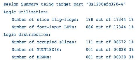
The design is fully pipelined and can provide new outputs in any one clock cycle. The delay is 10 clock cycles and the maximum data rate is 194.70MSPS (million samples per second). In terms of numerical accuracy, for a 1000 or 2000 word ILUT, the ratio of the reference floating point result to the quantization error of the System Generator for DSP fixed point output, ie, the signal to noise ratio is 71.94 dB or 77.95 dB, respectively.
In addition to ILUT, we can also use the CORDIC SQRT module in the Reference Math Blockset provided by Xilinx System Generator for DSP. In this example, the total delay is 37 clock cycles, the maximum data rate is 115.18 MSPS, the area resource occupancy is 940 flip-flops, a total of 885 four-input LUTs, 560 occupied chips and two MULT 18x18 embedded Multiplier. The signal to noise ratio is 40.64 dB. These results show that CORDIC is an ideal way to implement fixed-point math, but ILUT is better in many ways.
Single Mode Fiber Patch Cord is a single stand of glass fiber with a diameter of 8.3 to 10 microns that has one mode of transmission. Single Mode Fiber with a relatively narrow diameter, through which only one mode will propagate typically 1310 or 1550nm. Carries higher bandwidth than multimode fiber, but requires a light source with a narrow spectral width. Synonyms are mono-mode optical fiber, single-mode fiber, single-mode optical waveguide, uni-mode fiber.
Single-mode fiber gives you a higher transmission rate and up to 50 times more distance than multimode, but it also costs more. Single-mode fiber has a much smaller core than multimode. The small core and single light-wave virtually eliminate any distortion that could result from overlapping light pulses, providing the least signal attenuation and the highest transmission speeds of any fiber cable type.Single-mode optical fiber is an optical fiber in which only the lowest order bound mode can propagate at the wavelength of interest typically 1300 to 1320nm
Single Mode Fiber Patch Cord
Single Mode Fiber Patch Cord,Single Mode Patch Cord,Single Mode Patch Cable,Fiber Optic Patch Cord
Foclink Co., Ltd , http://www.scfiberpigtail.com