Since the early 20th century, thermocouples have been widely used for critical temperature measurements, especially in the extremely high temperature range. For many industrial and process critical applications, T/C and RTD (resistance temperature detectors) have become the "gold standard" for temperature measurement. Although RTDs have better accuracy and repeatability, thermocouples have the following advantages:
• Large range
• Fast response time
• Lower cost
• Better durability
• Self-powered (no excitation signal required)
• No self-heating effect
However, the use of thermocouples for high precision temperature measurements can be complicated. You can optimize measurement accuracy with solid circuit design and calibration, but understanding how thermocouples work can help you design your circuit or use a thermometer.
When a voltage source is applied to a length of wire, current flows from the positive end to the negative end, and the wire heats up, causing a portion of the energy loss. The Seebeck effect discovered by Thomas Seebeck in 1821 is a reversal: when a temperature gradient is applied to a length of wire, an electric potential is generated. This is the physical basis of the thermocouple.
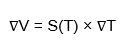
(Formula 1)
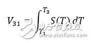
Where ∇V is the voltage gradient, ∇T is the temperature gradient, and S(T) is the Seebeck coefficient. The Seebeck coefficient is material dependent and is also a function of temperature. The voltage between two different temperature points on a length of wire is equal to the integral of the Seebeck coefficient function over temperature.
(Formula 2)
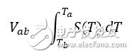
For example, T1, T2, and T3 in Figure 1 represent the temperature at different points on a length of wire. T1 (blue) indicates the lowest temperature point and T3 (red) indicates the highest temperature point. The voltage between T2 and T1 is:
(Formula 3)
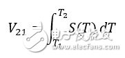
Similarly, the voltage between T3 and T1 is:
(Formula 4)
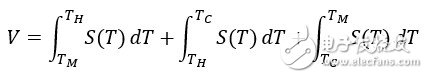
According to the additivity of the integral, V31 is also equal to:
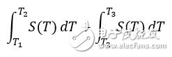
(Formula 5)
We will keep this in mind when discussing the voltage and temperature transitions of thermocouples.
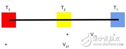
Figure 1: According to the Seebeck coefficient, the temperature gradient produces a voltage across the conductive metal.
The thermocouple consists of two different metals, and the Seebeck coefficient S(T) of the wire is generally different. Since a temperature difference across a metal can create a voltage difference, why do you have to use two metals? It is assumed that the wire in Fig. 2 is made of the material "A". If the probe of a voltmeter is also made of material A, in theory, the voltmeter will not detect any voltage.
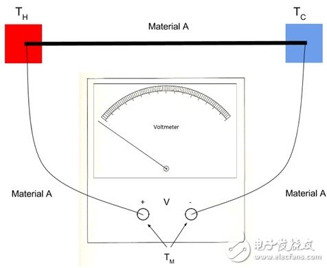
Figure 2: Voltage measurement connection. When the material of the probe and the wire are the same, there will be no potential difference.
The reason is that when the probe is attached to the end of the wire, it is equivalent to extending the wire. The two ends of the long wire are connected to the input of the voltmeter with the same temperature (TM). If the temperatures at both ends of the wire are the same, no voltage is generated. To prove this mathematically, we calculate the voltage accumulated across the metal ring from the positive to the negative side of the voltmeter.
(Formula 6)
According to the additivity of the integral, the above formula becomes:
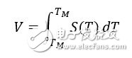
(Formula 7)
When the lower and upper boundaries of the integral are the same, the result of the integration is V=0. If the probe material is B, as shown in Figure 3, then:
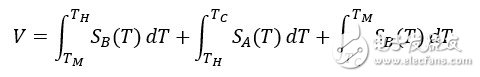
(Equation 8)
Simplify the above formula, we get:
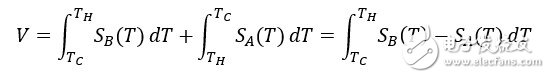
(Equation 9)
Equation 9 shows that the measured voltage is equal to the integral of the difference between the Seebeck coefficient functions of the two materials. This is why thermocouples use two different metals.
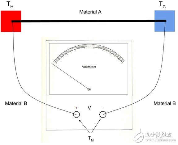
Figure 3: Voltage measurement connection. The probe and wire are made of different materials, illustrating the physical reality of the Seebeck coefficient.
Material A: Material A
Material B: Material B
Voltmeter: Voltmeter
According to the circuit in Figure 3 and Equation 9, assuming that SA(T), SB(T), and the measured voltage are known, we still cannot calculate the temperature (TH) of the hot end unless we know the temperature (TC) of the cold junction. In the early stages of the thermocouple, a freezing point furnace at a temperature of 0 °C was used as the reference temperature (the term "cold end" is thus derived) because this method is low in cost, easy to implement, and capable of self-regulating the temperature. The equivalent circuit is shown in Figure 4.
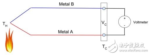
Figure 4: The thermocouple requires a reference temperature, 0 °C as shown, to calculate the unknown temperature TH.
Although we know the reference temperature of the circuit shown in Figure 4, it is not practical to obtain TH by integration. Then there is a standard reference table that supports common thermocouple types, and the corresponding temperature of the corresponding voltage output can be obtained by looking up the table. However, it must be borne in mind that all standard thermocouple reference tables are drawn with 0°C as a reference point.
Thermocouple systemModern thermocouples consist of two different wires joined together by one end (TH). The voltage is measured at the open end of the wire pair. According to the equivalent circuit shown in Fig. 5, VC is the same as Equation 9 in Fig. 3 above.
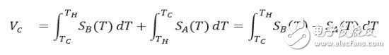
(Formula 10)
Figure 5: Modern thermocouple configuration with cold junction compensation.
The cold junction compensation cold junction (TC) temperature can be set to 0 °C of the freezing point furnace, but in practical applications, we do not use the ice bucket as the reference temperature. Using the CJC (cold junction compensation) method, the hot junction temperature can be calculated without using the 0 °C cold junction temperature. Even the cold junction temperature is not necessarily constant. This method uses only a single temperature sensor to measure the temperature at the TC point. If TC is known, TH can be obtained.
If we use a temperature sensor to measure the cold junction temperature, why not use this sensor to directly measure the temperature of the hot end? As you can see, the cold junction temperature range is much narrower than the hot end temperature range, so the temperature sensor does not need to support the extreme temperatures supported by the thermocouple.
Calculate hot end temperature using CJC
As mentioned above, all standard thermocouple reference tables are obtained at 0 °C at the cold end. So how do you use the reference table to get the hot end temperature? Imagine extending the open end of the above thermocouple and connecting the imaginary end to a junction with a temperature of 0 °C (Figure 6). If we can calculate the V0 value, it is easy to get the corresponding hot end temperature using the reference table.
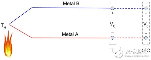
Figure 6: Connecting the extended thermocouple to the 0°C junction determines the unknown hot junction temperature TH.
Determine V0
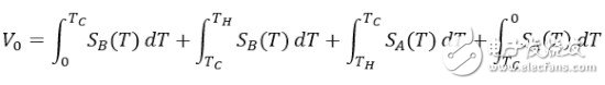
(Formula 11)
Rearrange the above formula:
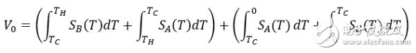
(Formula 12)
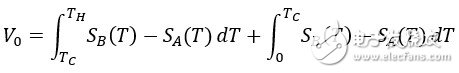
(Expression 13)
(Expression 14)
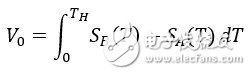
The first term of Equation 13 is identical to Equation 10 (obtained from Figure 5). The equivalent voltage output is VC, which is a known value because the temperature at the cold junction is measured by a voltmeter. The second term is equivalent to the output of the thermocouple when the hot end temperature is equal to TC and the cold end temperature is equal to 0 °C. Since the TC is also measured by an independent temperature sensor, we can use the standard reference table to find the corresponding Seebeck voltage (Vi) for the second term in Equation 13:

(Equation 15)
Using the V0 value, the corresponding temperature at TH can be determined by a standard reference table.
The process of calculating the hot end temperature using cold junction compensation is divided into the following steps:
• Measure the cold junction temperature (TC) with a temperature sensor.
• Measure the cold junction temperature.
• Convert TC to voltage (Vi) via a standard reference table.
• Calculate V0=Vi+VC.
• Convert V0 to temperature TH via a standard reference table.
The standard thermocouple reference table can be found in the NIST ITS-90 Thermocouple Database. If the lookup table cannot be implemented in the microcontroller due to memory or other reasons, the NIST ITS-90 website also provides a set of formulas for each type of thermocouple that can be used to convert between temperature and voltage.
System design pointsSo far, the above discussion has been limited to the theoretical knowledge of thermocouples. In order to optimize the accuracy of the actual system, there are several things to note. Each device in the basic thermocouple signal chain (Figure 7) will affect conversion accuracy and must be carefully selected to minimize errors.
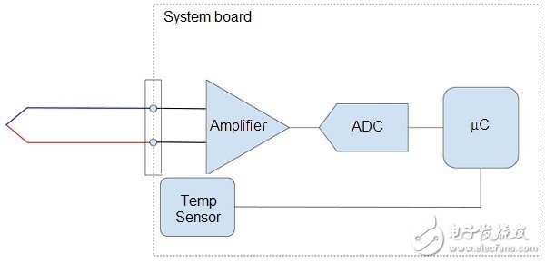
Figure 7: The basic components of a thermocouple measurement system include an amplifier and an ADC, and a microcontroller that can then calculate the unknown temperature.
System board: System board
Amplifier: Amplifier
Temp sensor: Temperature sensor
Starting from the left side of Figure 7, the thermocouple is connected to the connector of the system board. The thermocouple itself is also a sensor or a source of error. Longer thermocouples can easily pick up electromagnetic noise from the surrounding environment; shielded wires can effectively reduce noise. The next component is the amplifier, which has a high input impedance and is important because the amplifier's input impedance and thermocouple resistance form a voltage divider. The higher the input impedance of the amplifier, the less error it produces.
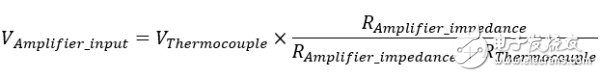
(Formula 16)
In addition, the amplifier increases the thermocouple output and the thermocouple output is typically in the millivolt range. Although the amplifier's high closed-loop gain amplifies both signal and noise, adding a low-pass filter to the ADC input eliminates most of the noise. Because temperature changes are not very fast, the ADC conversion rate for such applications is typically very low—perhaps only a few samples per second—so the low-pass filter is very efficient.
Finally, the onboard temperature sensor needs to be very close to the cold junction connector (ideally in contact with the end of the thermocouple wire, but in many cases the conditions are not allowed) to obtain the best cold junction temperature measurement. Any errors in the cold junction measurement will be reflected in the hot junction temperature calculation.
Thermocouple circuit examples and test resultsWhether you design your own thermocouple measurement circuit or a reference design, you need to verify its accuracy. The accuracy verification of the MAXREFDES67# reference design (Figure 8) is described below.
Figure 8: The MAXREFDES67# is a reference design for thermocouples and RTDs that measures voltage and current to measure temperature from -40°C to 150°C.
To illustrate how to minimize measurement errors, we first take a thermocouple system, such as Maxim's MAXREFDES67 reference design. In order to verify the error of the measurement system or any measurement system, a known temperature and a reliable instrument is required for comparison. In this example, we used three reference thermometers: the Omega HH41 thermometer (now replaced by HH42), the ETI reference thermometer, and the Fluke 724 temperature calibrator. A Type K thermocouple connected to the MAXREFDES67# was placed in a Fluke 7341 calibration furnace and calibrated at 20 °C. The blue dot data is referenced by Omega HH41, and the green dot data is referenced by the ETI device. The red dot data shows a maximum error of less than 0.1 °C, based on the Fluke 724 calibrator, but unlike previous tests, the Fluke 724 is not used as a reference instrument. Simulate the ideal K-type thermocouple output and connect the input of the MAXREFDES67# to the thermocouple extension cable. Figure 9 shows the test results.
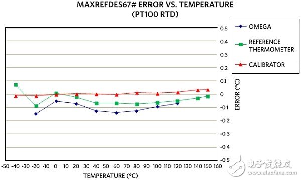
Figure 9. Using the Omnitec EC3TC (K-type thermocouple, calibrated at 20 °C), evaluate the MAXREFDES67# error vs. temperature and compare it to the other three reference thermometers. The results show that very high precision is achieved.
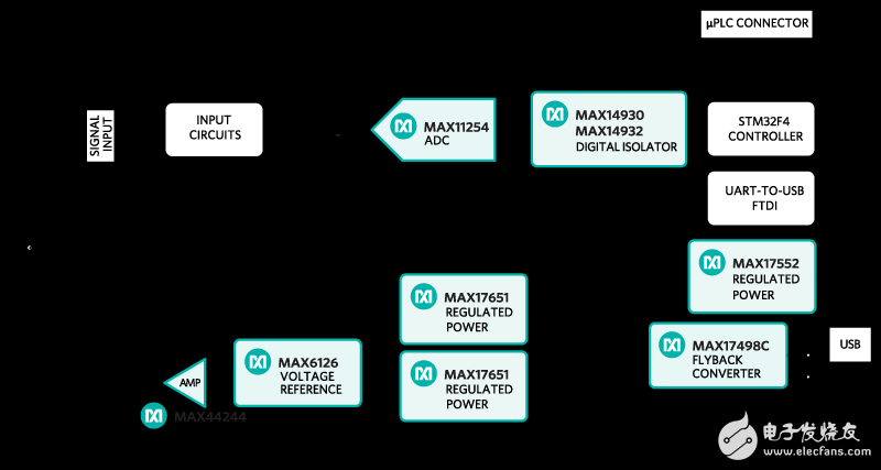
Figure 10: Block diagram of the MAXREFDES67# reference design.
to sum upThermocouples offer many advantages in industrial temperature measurement applications, including temperature range, response time, cost, and durability. The thermocouple theory is slightly more complicated, but we must fully understand it so that it can perform correct measurements and high-precision conversion from voltage to temperature. The MAXREFDES67# reference design uses the MAX11254 and MAX6126 chips, making it ideal for temperature-sensitive small-signal, high-precision measurement applications such as thermocouple temperature measurement. Among them, MAX11254 is a 6-channel, 24-bit, delta-sigma ADC, which achieves low noise and high precision while reducing power consumption by 10 times. The MAX6126 is an ultra-low noise, ultra-high precision, low dropout series voltage reference. The temperature coefficient is 3ppm/°C (maximum) with excellent ±0.02% (maximum) initial accuracy.
Electronic Vapor Cigarettes,Wholesale Disposable Vape Pen,Disposable E Cig,Cigarette Electronic
Maskking(Shenzhen) Technology CO., LTD , https://www.szelectroniccigarette.com